Block Diagrams in LaTeX
About
This post assumes that you are already familiar with
LaTeX. You know how to wite tex documents
and how to compile them into PDFs.
If you don’t have a working environment for compiling tex documents, you can use Overleaf in your browser to practice.
The intention of this post is to provide a high-level introduction of the TikZ package and explain the basics to get you started with simple drawings. It is not meant to be a comprehensive guide for its full use. For more details on how to use the TikZ package, you can refer to the Reference section. As you go through this tutorial, keep in mind that there are multiple ways to accomplish the same. This guide provides a different path for drawing your diagrams.
Why TikZ?
TikZ is a powerful LaTeX package that allow us to maintain the elegance of
our documents with aethetically-pleasing drawings. Namely, TikZ allows us to
draw diagrams and plots by coding the specific positions and styles we want to
use.
Someone put together a list of available TikZ libraries with some general descriptions. Some examples include:
- drawing block diagrams and flowcharts,
- a paper folding library, and
- structural analysis.
This post will provide a bit of insight towards drawing block diagrams and flowcharts.
Download this file
I provide a sample tex file (named tikzplayground.tex) that you can use as a
starting point. You can use it within your environment or copy the text into
Overleaf. You should be able to compile it and generated the pdf out of the
box. This post will reference this sample file throughout the examples.
Getting Started
To start using the TikZ libraries, first include the relevant packages in your tex file.
\usepackage{tkz-euclide}
\usepackage{tikz}
Use the \usetikzlibrary{} command to include the specific library you want to
use. Our sample file calls the following libraries for drawing block diagrams
and flowcharts:
\usetikzlibrary{arrows}
\usetikzlibrary{quotes,angles}
\usetikzlibrary{positioning}
\usetikzlibrary{plotmarks}
\usetikzlibrary{shapes.geometric, arrows}
You can then start constructing your diagram as a figure by including the following to your tex file:
\begin{figure}[h]
\begin{center}
\begin{tikzpicture}[auto, node distance=2.7cm, >=latex']
... code ...
\end{tikzpicture}
\end{center}
\end{figure}
The following sections describe the code you need to add by replacing the
... code ... section to draw block diagrams and flowcharts.
Define Styles
Before we start drawing, let’s define some styles first. This is optional but I’ve found it really helpful to define the style/dimensions of your drawing blocks such that you can just reference them by type in your overall drawing. These will be the building blocks for your diagrams.
For example, the following defines a rectangular block that can later be
referenced in the code by block. Specifically, it defines the shape, its
dimensions, the position of the text, and the color and fill of the box:
\tikzstyle{block} = [rectangle, minimum width=2.5cm, minimum height=1cm, text centered, text width=2.7cm, draw=black, fill=white]
Similarly, the following defines a circular block that can be referenced in the code by “sumation”:
\tikzstyle{sumation} = [circle, minimum width=0.2cm, minimum height=0.5cm, text centered, text width=0.4cm, draw=black, fill=white]
There are more building block examples in the provided tikzplayground.tex file.
Block Diagrams
Simple Feedback Diagram
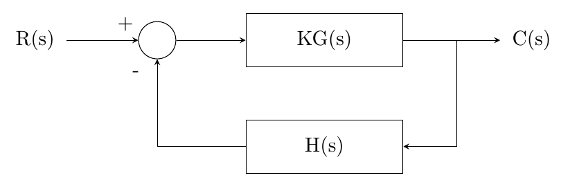
Refer to Section 1 in the provided tikzplayground.tex file. The following block diagram describes the transfer function of a noise-free physical linear system:
The code to draw diagrams is composed of two main parts: 1) draw the nodes and their positions, and 2) draw the arrows/lines to connect the nodes.
Let’s look at an example. Let’s add the sumation circle to the right if the
R(s) input (where sumation is a style that is defined at the top of the tex
file):
  \node (input) [circle] {R(s)};
  \node (sum) [sumation, right of=input, xshift=-0.4cm] {};
inputandsumare the internal names of each node. It’s how the diagram references each node.circleandsumationare the node types.right of=andxshift=is how we specify exactly where we want each node. Each node is positioned relative to another except the first one.- Text inside the bracket at the end (
{}) is the text that will be added next to the corresponding node.
Now let’s connect the sum and input with an arrow:
\draw [arrow] (input) -- node[anchor=north] {} (sum);
This line draws an arrow from the input node to the sum node. The two
dashes (--) specify that we’re drawing a straight arrow (more complicated
examples in the next section). If we wanted to add text to the arrow, we could
have included text inside the brackets in [anchor=north] {}. The cardinal
direction defined by “anchor” determines where the text will be drawn.
More complicated connections
The TikZ package automatically decides where to draw the base and tip of the arrow. The default is when the nodes are next to each other (e.g., side to side or one is above or below the other).
The beautiful thing about TikZ is that we have more control over the lines. For
example, the following line (used to draw the block diagram above) uses the
convention -| to determine the order and direction of the arrows between the
hs and sum nodes:
\draw [arrow] (hs.180) -| node[anchor=north] {} (sum.270);
The convention -| specifically says “first draw a horizonatal line and then
a vertical one.”
Morever, we can specify the start and end points of the connecting arrow. Imagine that each node is encompassed inside a unitary circle (shown below), which follows the angle convention of 0 ° facing to the right, 90 ° facing upwards, 1800 ° facing to the left, etc.
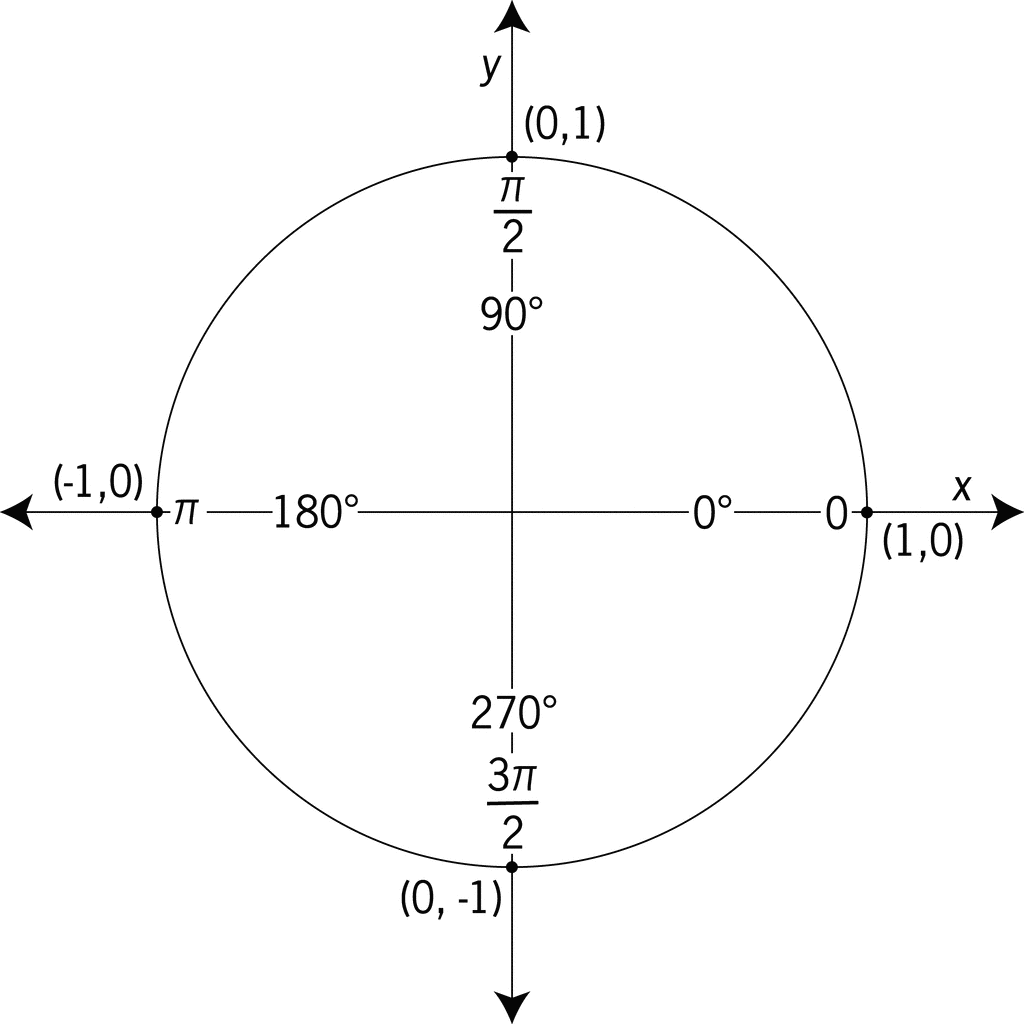
We can use this angle representation to specify specific locations around the
circle. For the block diagram above, we want the arrow to start at the left of
the H(s) block and end at the bottom of the sum block. As such, as the line
above specifies, we start the line at (hs.180), which is 180 ° of the
H(s) block and (sum.270), which is 270 ° of the sum block.
Having this control on where exactly to place arrows and lines comes in handy when we’re structuring more complicated drawing. See the General Drawings section for specific examples.
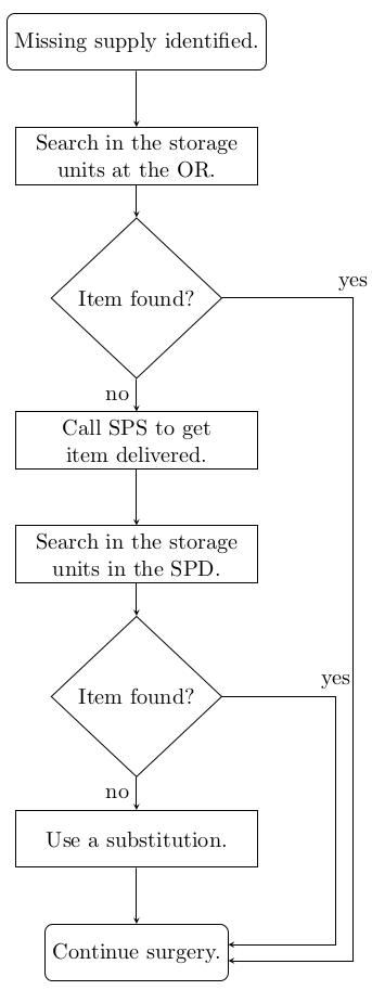
Flowcharts
Drawing flowcharts is very much the same as block diagrams. The same nodes and arrows concepts apply.
Refer to Section 2 in the provided tikzplayground.tex file. You’ll see the code for the flowchart below:
General Drawings
This is where TikZ gets interesting. Checkout these funky figures we can draw. We can add textures (like water), and we can precicely place labels to specific points in the drawings.
Refer to Section 3 in the provided tikzplayground.tex file.
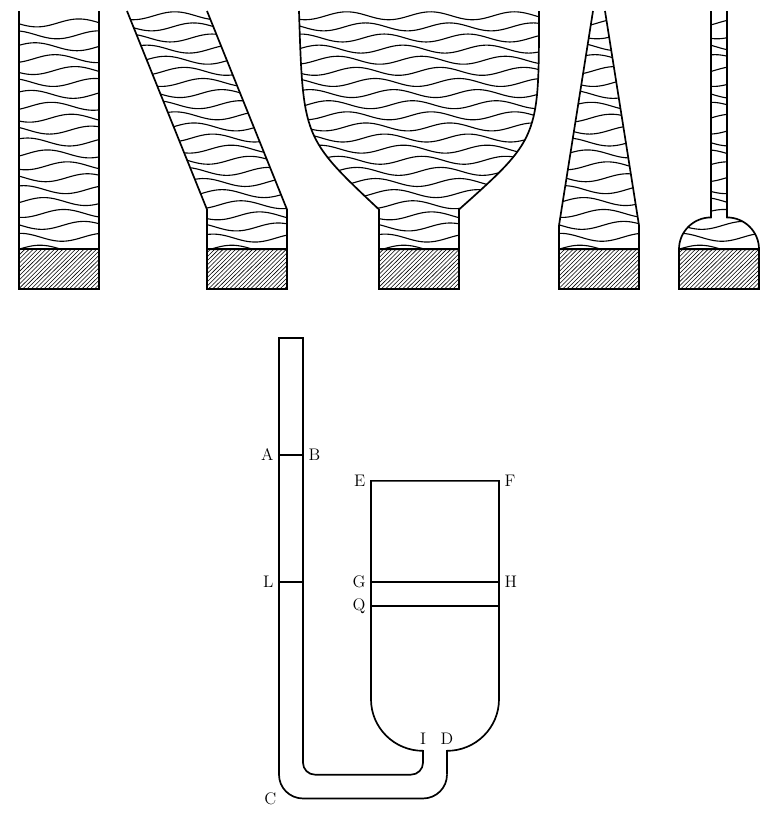
One important takeaway from this section is that we can specify exactly where we want each line, point, label, etc. TikZ offers a mathematical way of drawing exactly what we want.